
Predators and Prey
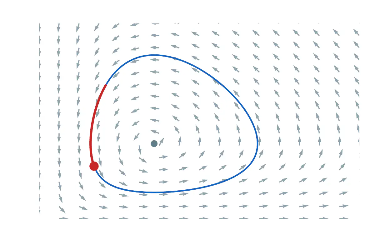
The Lotka–Volterra model in the plane of the two populations: a direction field, the closed orbit of a solution, and a state that an action moves around it.
A population of prey x grows when it is left alone, and is eaten at a rate proportional to the number of meetings between prey and predators. A population of predators y dies out when it is left alone, and grows with the same meetings. Alfred Lotka (1925) and Vito Volterra (1926) wrote this as x' = ax - bxy and y' = dxy - cy .
The picture is the plane of the two populations, not a plot against time. At each point the arrow shows where the populations go next. Many prey feed more predators; many predators leave few prey; few prey starve the predators; few predators let the prey recover. So the state turns around the equilibrium \left(\frac{c}{d}, \frac{a}{b}\right) , the grey dot inside the orbit, where both populations stay constant.
In this model the state returns exactly to its start: the quantity V(x, y) = dx - c\ln x + by - a\ln y does not change along a solution, so each solution is a closed level curve of V . The blue curve is the level curve through the start (p, q) . An action moves the state along it with the fourth-order Runge–Kutta method, h = 0.03 time units every 30 milliseconds. Edit the rates a , b , c , d or the start p , q (all six must stay positive), then run the second action to put the state back at the start. Near the equilibrium one turn takes the time \frac{2\pi}{\sqrt{ac}} ; a larger orbit takes longer.
After a JSXGraph example by The Center of Mobile Learning with Digital Technology.
JavaScript is required to view the interactive plot.